Temporal difference reinforcement learning has been successfully used to teach a multi-layer perceptron to learn to play backgammon through self-play. In this project I have applied the same technique to the game of cribbage. Because cribbage contains lots of reinforcement information, it suggests that a multi-layer perceptron network can learn quickly. By varying the parameters of the algorithm I can see how changing them affect how well the network learns, and how fast the network learns.
Tesauro has demonstrated that temporal difference (TD) learning can be be used to train a multi-layer perceptron to play backgammon though self-play. A two-layer perceptron with 40 hidden units was trained by playing against itself for tens of thousands of games. In the end, the perceptron network could beat Sun’s Gammontool program 65% of the time, and could beat Neurogrammon 1.0, 50% of the time. This ranked the program well into the intermediate level of play for humans.
Moves were chosen by picking a legal move that put the player into a state with the highest utility value as determined by a utility function. The multi-layer perceptron represented this utility value. During training, the network was trained by the TD learning algorithm made it more accurately represent the actual utility of game states.
These results are very encouraging because, a priori, there is no reason to believe that TD learning can train a utility function in this situation. As the network learns, it adjusts its playing strategy, and the opponent (itself) learns as well and changes its strategy. The probability distribution of moves of the opponent adjusts, so the utility function that is being trained also changes. Because the utility function changes as the network learns it, we have no reason to believe TD learning would even converge, let alone converging to an optimal value.
Another potential problem is over-training. One reason that this may occur, is that a more accurate utility function may lead to worse play. When determining what move to make, only the relative values of utility function for the possible moves are important. As long as the best move has the highest value, the correct move can be made. If two moves have almost the same utility value, then it is possible for a more extensively trained network to have more accurate utility values, but have the difference between them negated. This can cause more accurate network to choose a worse move then would a less accurate network that happens to have the difference with the correct sign.
Play in cribbage is divided into several hands. In each hand, players are given a set of six cards, and must discard two. Then player alternate playing their hand, and scoring points based on the sequence played. Then finally the hands are scored, and the crib, composed of the discarded cards, is scored for the dealer. The first player to reach 121 points wins.
Cribbage has several advantages that, hopefully, will make it easy to learn. Because points are scored during play of a hand, and many points are scored at the end of a hand, there is lots of reinforcement available. In other games, like backgammon, there is only a binary reward at the end of the game. Also the hands of cribbage are relatively short, so little computer time is need to play many hands.
The most important difference between cribbage and backgammon is that the state of the game is not completely known, and the initial state is chosen at random. I do not feel that this will cause any problems, because one can think of the state as entirely known, with random branches during play. These random branches are the results of the opponent's previously unknown cards being exposed. This process should be no different than the random process of rolling dice during play in backgammon.
I should note that the optimizing score is not necessarily best strategy in cribbage. The goal is to be the first to score 121, so near the end of the game it may be more important to score points during play, to get to 121 first, and sacrifice scoring even more points later. For the purposes of this program, we will ignore this small effect, and work on maximizing the scores of each hand.
A simple discard game was also the subject of investigation in the project. This is like a simplified version of cribbage. There is no play involved. A player is dealt six cards, and then asked to discard two of them. The remaining four cards are score along with a random start card according to the scoring rules for hands in cribbage.
This simpler game is used as an intermediate step in determining the feasibility of using multi-layer perceptrons to learn the game of cribbage. If a multi-layer perceptron can not even learn this simple game, then there would be little hope of it learning the full game of cribbage. However, if it can learn this game, then it provides incentive to try learning the full game of cribbage.
The baseline method to compare the multi-layer perceptron with was random play. A random legal move is selected for play.
The AI algorithm uses a multi-layer perception to represent a utility function of a given state. The AI algorithm selects the move that puts the AI player into a state that maximizes the predicted utility of the multi-layer perceptron. A state is represented by a vector of 209 inputs that are each set to 0 or 1. One input represents if the player is dealer or not. 52 inputs represent the hand. Each input represent one card. The input is 0 if the card is not in the hand, and 1 if the card is in the hand. Another 52 inputs represent the other known cards, including the known part of the crib, and the start card. The last 104 inputs represent the state of play. The first 13 represent the rank of the first card played, the second 13 cards represent the rank of the second card played, and so forth.
The multi-layer perceptron was trained using the temporal difference learning algorithm. During play the multi-layer perceptron value for a given state is trained to be the reward for that state (the points earned when the player entered the state, or minus the points earned by an opponent) plus the predicted utility of the successor of that state. The final state is trained to be the the reward for that state (the difference between the points earned by the player and the opponent). To be more precice the temporal difference learning algorithm after observing a transition from state i to state j is
where w is a vector representing the weights in the multi-layer perceptron, α is the learning rate, r is the difference of the points the player gained and the points the opponent gained in state i, Uw is the utility function. After each player move, the multi-layer perceptron is updated using this equation.
The multi-layer perceptron was initialized with random values from a Gaussian distribution with mean 0.0 and with a standard deviation of 1.0. The multi-layer perceptron had only one hidden layer which had a variable number of nodes. The nodes all utilized a sigmoid transfer function ((1 + e-x)-1), except for the final node which was a linear output node.
The multi-layer perceptron was trained using the standard back-propagation algorithm. This does a gradient descent search to update the weight values. This method requires a learning rate parameter. This parameters was a variable parameter.
During the learning process, the AI program played another instance of the same program that shared the same multi-layer perceptron. So as play proceeded, both players trained the network, and therefore as play proceeded, the AI player’s opponent (himself in some respects) became more intelligent. This means that the AI program cannot rely on the lack of intelligence of his opponent to score more points.
Similar algorithms were used for the simple discard game. Since there is only one move, Temporal difference was not exactly used. However the value of the final state was trained independently from other sessions, just as what happens with temporal difference learning. Also the inputs were simplified to just 52 inputs representing the hand.
Two other algorithms were used for the simple discard game. One algorithm cheated by looking at the start card, and discarded the two cards that maximized the number of points received. This was the maximum possible score any player could achieve for this hand. The other algorithm was perfect algorithm. It discarded the two cards that would produce the highest average scored based on the possible cards that the start card could be. This represented the best that I could hope the AI algorithm could play.
There are several other approaches to program a computer to play cribbage. One approach is to use a search tree to find optimal move for a given situation. Various heuristics could be used to speed up play. It is possible the game is simple enough that a full search could be done.
I suspect that such an approach would be more difficult to write. The value of using a multi-layer perceptron is its simplicity. The java code used is about 1 000 lines long.
One could use supervised learning on expert data. In this method, moves are solicited from expert cribbage players for given positions in the game. One could train a neural network on this information.
This approach requires an expert who know how to play cribbage well. Gathering training data from an expert would be a long and expensive procedure. After training we can only hope that the neural network can generalize what it has learned to other situations. Such generalizations may fail. Also we cannot be sure how close the expert moves are to ideal moves, and we therefore limit ourselves to being no better than the human expert.
One could simply encode a particular strategy that a person uses to play cribbage. After playing many hands of cribbage it becomes clear how to play in most situations. One could consult with an expert cribbage player and explicitly write out the algorithm used by that person.
The drawbacks of such an approach is that one needs to know how to play cribbage beforehand. Such an approach probably will not lead to ideal play. It would also be difficult for an expert to explicitly describe his algorithm for playing cribbage. And finally, such an approach would be very difficult to program. One would have to ensure that every possible case is covered, so that the program always can choose a play.
My first tests were on the neural network, to test to see that the back propagation algorithm was working correctly. I attempted to teach a multi-layer perceptron a constant function, a linear function (x + y), and a non-linear function (sin(6x)/4 + x/2 + 1/4). The multi-layer perceptron for the constant function and the linear function both had two inputs and 10 hidden nodes with sigmoid transfer function, and a single linear output node. In both these cases, the neural network converged very quickly. The multi-layer perceptron for the non-linear case only had one input, but was otherwise identical. The non-linear function took longer to converge. But after about 5 million iteration, the mean square error was on the order of 10-4 (on the range [0 1]), and further iteration did not improve this error.
With successful results using the neural network, I applied it to the simplified discard game. I also tested the random algorithm, the cheating algorithm and the ideal algorithm. These algorithms do not learn, so I calculated their mean scores over 20 000 hands. The random algorithm scored 4.7 point on average. The ideal algorithm scored 8.1 points on average. The cheating algorithm scored 8.8 points on average.
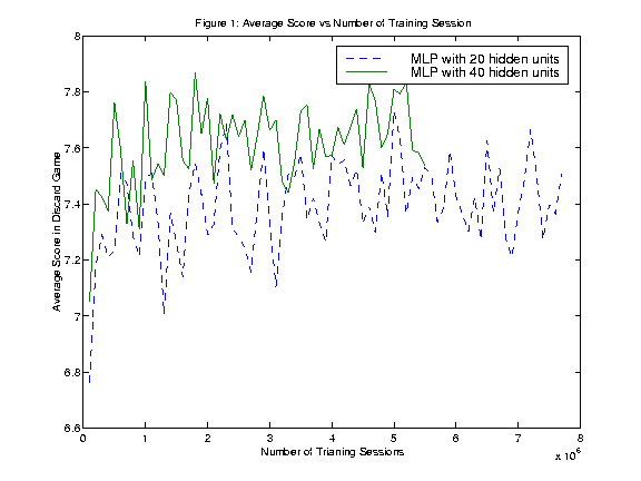
Figure 1 shows the results of training a multi-layer perceptron to play the discard game. Results for two networks were calculated. One network had 20 hidden nodes, and the other network had 40 hidden nodes. Both networks used a learning rate of 0.01. The results show that the networks can both quickly learn to score 7.3 to 7.6 points. Both algorithms quickly plateaued and little learning took place afterward.
The scores produced are reasonably close to the ideal score of 8.1. Perhaps with more hidden nodes, or with a different method of characterizing the inputs, a better score could be achieved. However these results are encouraging enough to attempt to learn the full game of cribbage.
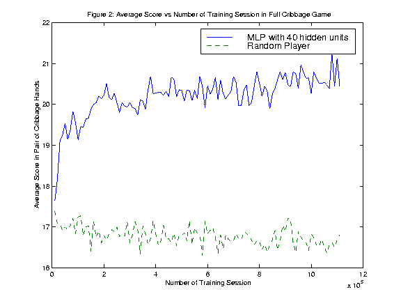
Figure 2 shows the results of training a multi-layer perceptron to play the full game of cribbage. The results took two days of computer time to calculate, and it seems clear that a peak has not been reached in that time. The graphs shows the scores of the pairs of hands of random player versus the AI player averaged over 1 000 pairs of hands. In each pair of hands each player got to be dealer once. Over the period of learning the AI player managed to learn to score around 4 points more that the random player.
This learning had been achieved through self play alone. The only knowledge that the AI was initially programmed with was what moves were legal.
Now that one knows that this approach leads to some learned intelligence, the next step would be to compare this approach to human ability. This comparison is labour intensive to perform. Because scores in cribbage are fairly highly dependent on luck, many many games would need to be played to get a fair comparison. Due to time constraints, such a comparison could not be performed for this paper.
One would also be interested in comparing this approach to other cribbage programs. It is probably feasible to write a program that does a perfect job at maximizing the score for a hand. Writing this program and comparing this AI cribbage program to it would give a very good comparison allowing us to determine the quality of play.
Several variations of this algorithm should be explored. Comparing how fast and well this procedure works when different learning rates and different number of hidden nodes are used would be useful to know. What would also be of interest is varying the number of hidden layers used to see what effect this would have.
Other variations of this algorithm that should be explored involve changing the input representation. The input representation chosen is close to the raw information available from the game. However, in most games performance can be affected by applying a transformation to the inputs. If the inputs are based on features of the play that we know are important (from experts in cribbage), then learning can be improved.
Another variation worth trying is the TD(λ) algorithm. The formula for the TD(λ) learning assigned some of the utility of much later game states to earlier game states, where as the normal TD algorithm only assigns the utility of a state to its immediate predecessor. For a given state, its utility is assigned to all its predecessor with a weight of λn, where n is the distance between the states. Such an approach can often speed up the learning process.
Using self-play to train a multi-layer perceptron has been successful in learning several games. Exploring the limits of this approach with other games would be useful. But a mathematical justification for this approach would be even better. So further research into understanding the mathematics behind this should be undertaken. With a better mathematical understanding we would be able to know the limitations of this approach. However, I expect the mathematics to be very difficult problem to tackle.